


We treat outliers in survey data as a staged production problem, not a single delete-or-keep decision: data cleaning, imputation, and estimation each demand different diagnostics and different fixes. We correct genuine errors where the evidence supports it, set truly suspicious values to missing and impute them, or protect final estimates through robust methods and weight calibration, always documenting the choice and checking it with a sensitivity analysis. Because survey weights, stratification, and clustering change how influence is measured, a value’s design weight matters as much as its raw size.
TL;DR:
- Outlier handling in surveys requires stage-specific fixes: correction for errors, robust imputation for true extremes, and influence-based adjustments during estimation.
- Multiple detection methods, including univariate, multivariate, and machine learning, must be layered and validated, especially for skewed or zero-inflated variables.
- Influence diagnostics must account for survey design by considering weights and clustering, with high-influence units treated through trimming, calibration, or sensitivity analysis.
- Flagged values should follow clear decision rules: fix errors, impute plausible data, or apply weight-aware adjustments, with each step well documented.
- Recontact and paradata analysis help verify flagged cases, and cascading flags combined with sensitivity testing ensure credible estimates.
Table of Contents
- Workflow for Outlier Handling in Survey Production
- Detection Methods for Spotting Outliers in Survey Data
- Survey-Aware Influence Diagnostics and Weight Considerations
- Treatment Options and Decision Rules for Flagged Values
- A Step-by-Step Checklist for Reviewing and Documenting Outliers
- Software and Code Direction for Implementation
- How Veridata Insights Supports Defensible Outlier Handling
- FAQ
- Sources
Workflow for Outlier Handling in Survey Production
Most of the confusion around outliers comes from treating them as one category of problem when they are really three. The RAND review of outlier detection and editing procedures frames this correctly: outlier handling in official statistics unfolds across data cleaning, imputation, and final estimation, and each stage asks a different question of the same flagged value.
At the cleaning stage, the question is whether a value is simply wrong. A respondent who reports an age of 333 or a household income entered in the wrong currency unit is not giving you a real extreme value, they are giving you a keying error or a unit mismatch, and the fix is correction, not statistical adjustment. The Boise State survey design guidance contrasts a plausible age like 55 against an impossible entry like 333 precisely because that distinction drives the entire downstream workflow: implausible values get corrected or queried before anything else happens to them.
At the imputation stage, the question shifts. A value might be perfectly real and perfectly extreme, a small business owner reporting revenue ten times the sample median, for instance, and deleting it would throw away genuine signal. Here the priority is protecting the imputation model from being distorted by that one case while still using the surrounding, trustworthy data to fill any genuine gaps. Robust multivariate methods matter most here because they let you estimate means and covariances even with missing values present, rather than letting a handful of odd cases warp the whole imputation model.
At the estimation stage, the question changes again: not “is this value wrong” or “is this value extreme” but “how much does this value, combined with its design weight, move my final number.” A valid extreme value attached to a small weight barely matters. The same value attached to a large design weight, representing many unsampled population units, can dominate a total or a mean on its own. This is the expanded contribution problem, and it is specific to survey estimation in a way that general statistics textbooks rarely address.
Moving a case between stages is itself a documented decision, not an afterthought. A value flagged during cleaning as “implausible” might get reclassified as “valid but extreme” once a recontact confirms it, or once paradata, like a completion time or device log, shows the respondent engaged carefully. The reverse happens too: a value that looked fine in cleaning might get flagged again at the estimation stage once its expanded contribution turns out to be unusually large.
A practical way to keep this straight:
- Cleaning stage: apply range and logic checks, correct obvious errors, flag anything implausible for review.
- Imputation stage: treat confirmed-valid extremes carefully with robust estimators so they do not distort imputed values for other cases.
- Estimation stage: compute expanded contributions, identify high-influence units, and apply weight-aware treatments before finalizing estimates.
Skipping a stage, or applying an estimation-stage fix like winsorization during the cleaning stage, is one of the more common ways analysts end up with defensible-looking numbers that do not hold up under review.
Detection Methods for Spotting Outliers in Survey Data
No single detection method covers every kind of problem a survey data set can throw at you, which is why a sound workflow layers several.
Univariate rules remain the fastest first pass. The interquartile range method flags values beyond 1.5 times the IQR from the nearest quartile, and simple z-scores or modified z-scores (based on the median and median absolute deviation) catch single-variable extremes quickly. Their weakness is exactly their simplicity: they treat each variable in isolation and say nothing about whether two values are jointly unusual, nor do they know anything about sample design.
Multivariate robust diagnostics close that gap. The RAND procedure uses a contaminated multivariate normal model estimated through the EM algorithm to compute Mahalanobis distances even when some values are missing, flagging both suspicious cases and the specific variables driving the flag. The R package modi implements multivariate outlier detection and imputation built around this same logic, which matters for survey variables that move together, like income and spending, where a univariate check on either variable alone would miss a case that is only unusual in combination.
Person-fit and response-pattern checks target a different failure mode entirely: not an extreme value but a disengaged respondent. Long strings of identical answers, implausibly fast completion times, and inconsistent logic across related items are signs of careless or insufficient-effort responding. Recent psychometric work on partial-carelessness detection argues against relying on a single time-per-item cutoff, recommending instead that timing, response-pattern, and person-fit indicators be combined, since careless responding is not one uniform behavior but a mix of patterns that a single threshold will not catch.
Machine-learning anomaly detectors add a further layer for larger or higher-dimensional data sets. scikit-learn’s outlier detection module documents IsolationForest and Local Outlier Factor as tools built around different assumptions: IsolationForest isolates anomalies through random partitioning, while LOF compares local density around a point to its neighbors. These methods answer a different question than a global statistical rule does, and the documentation itself is clear that algorithmic flags need validation against substantive checks rather than being treated as a verdict.
Where each method fits:
- Univariate rules (IQR, z-score, modified z): quick screening on individual variables, best as a first pass, not a final decision.
- Robust multivariate methods (Mahalanobis with robust covariance, RAND’s contaminated-normal and EM approach, modi): preferred when variables are correlated or missingness is present.
- Person-fit, timing, and long-string checks: aimed at careless or insufficient-effort responding rather than value-level extremes.
- IsolationForest and Local Outlier Factor: useful for larger or higher-dimensional data sets, but flags need substantive validation.
- Paradata cross-checks: completion time, device type, and navigation patterns help confirm or dismiss a statistical flag.
Combining timing, response-pattern, and person-fit indicators identifies careless responding more reliably than relying on a single cutoff, since careless response behavior takes several distinct forms rather than one uniform pattern. This is the core finding behind recent partial-carelessness detection research, and it is a direct argument against the common shortcut of flagging anyone who finishes “too fast.”
All of these methods share a blind spot worth naming directly: skewed or zero-inflated survey variables, common in income, spending, and health-utilization data, can trigger false flags under standard thresholds built for roughly symmetric distributions. An algorithmic flag or a 1.5xIQR cutoff is a starting point for review, never a stand-alone decision rule, and every flag deserves a look at the underlying paradata or a recontact before action is taken.
Survey-Aware Influence Diagnostics and Weight Considerations
A value’s raw size tells you very little in survey data until you multiply it by its design weight. This expanded contribution, weight times value, is the number that actually matters for a total or a mean, and it is also where ordinary outlier intuition breaks down. A moderate value with a huge weight can move an estimate more than an extreme value with a tiny one.
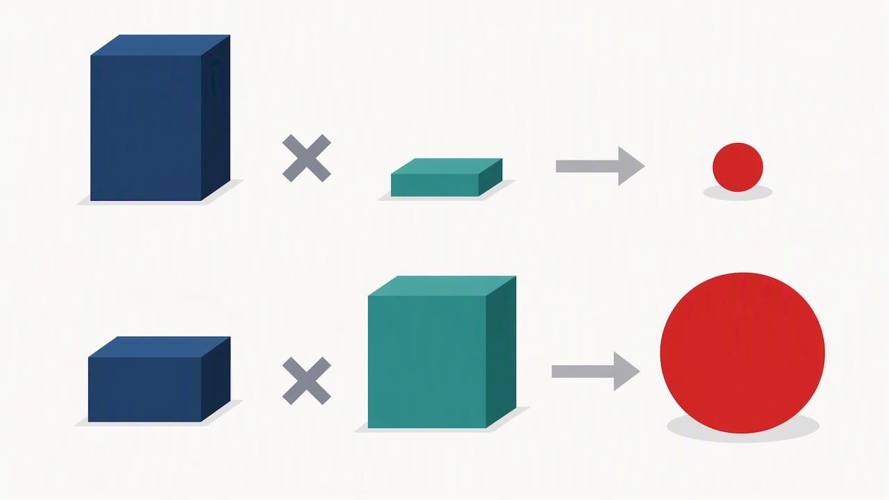
INSEE’s guidance on processing influential values draws a distinction that is easy to miss if you are coming from general statistics rather than official-statistics practice: a representative outlier is a genuinely extreme value that likely has counterparts elsewhere in the population, while a nonrepresentative outlier is a collection error masquerading as an extreme value. The treatment should differ accordingly. Representative outliers deserve weight-aware winsorization or conditional-bias methods that limit their influence without erasing the information they carry; nonrepresentative outliers are candidates for correction or removal, since they tell you nothing true about the population.
For regression-based survey analysis, ordinary influence diagnostics like DFBETAS, DFFITS, and Cook’s distance assume independent, identically distributed observations, an assumption complex samples violate by design. Survey-adapted versions of these diagnostics account for stratification, clustering, and unequal weighting, and they matter in practice: one documented case showed that correcting a single reporting error changed a wealth estimate substantially once the survey-aware influence diagnostic flagged it, a change a standard regression diagnostic would likely have understated.
Practical responses once a high-influence unit is confirmed:
- Weight trimming or calibration: cap extreme design weights or recalibrate them against known population totals, reducing the leverage of any single case.
- Weight-aware winsorization: cap the value itself at a threshold chosen with the weight distribution in mind, following approaches like Kokic and Bell winsorization referenced in INSEE’s methodology.
- Conditional-bias treatment: adjust the estimate based on the value’s contribution to bias rather than altering the raw data point.
- Documented retention: keep the value as reported and disclose its influence in a sensitivity table, appropriate when the case is genuinely representative.
Readers building out their own weighting approach may also find our breakdown of defensible survey weighting methods useful alongside this diagnostic layer.
Pro Tip: Before deleting or capping any flagged value, calculate its expanded contribution first. A value that looks alarming in isolation often turns out to carry a trivial weight, and vice versa.
Treatment Options and Decision Rules for Flagged Values
Every flagged value eventually needs a decision, and the decision should follow a visible rule rather than a case-by-case judgment call that is hard to defend later. INSEE’s guidance is explicit on this point: prespecified procedures and documented decision rules hold up to scrutiny, while ad hoc weight changes made value by value do not.
A workable decision sequence runs through four questions in order:
- Is the value impossible or logically inconsistent? Correct it if the true value can be determined, or set it to missing if it cannot.
- Is the value a likely data-entry or unit error? Correct it when a plausible true value is identifiable (a misplaced decimal, a unit mismatch), otherwise treat it as missing and impute.
- Is the value valid but extreme? Consider imputation using a robust model, a robust estimator for the statistic in question, or weight-aware winsorization, rather than deletion.
- Is the value influential for the specific estimand, regardless of how extreme it looks on its own? Apply weight trimming or calibration, or report the estimate alongside a sensitivity analysis that shows the result with and without the case.
Each treatment carries a trade-off worth stating plainly. Correction is the cleanest option when you can verify the true value, but it requires evidence, not guesswork, and guessing at a “corrected” figure without support is worse than leaving the flag undocumented. Imputation preserves sample size and avoids introducing nonresponse bias, but a poorly specified imputation model can quietly smuggle in the same distortion you were trying to avoid. Winsorization limits influence while keeping the case in the data set, which is often the most defensible middle ground for representative outliers, but the threshold choice itself needs justification rather than a default percentile picked without context. Weight trimming protects the overall estimate but changes the implied population the survey represents, so it should be applied sparingly and reported.
Running the full analysis with and without flagged cases included, and reporting both results, is standard practice in survey methodology for demonstrating that conclusions are not artifacts of a few unusual records. This single habit, the sensitivity analysis, does more to protect a study’s credibility than any individual detection method, because it shows reviewers exactly how much the treatment decision mattered.
Every action belongs in a written record: which variable, which rule triggered the flag, what evidence supported the decision, and what code produced the result. Analysts who skip this step are the ones who cannot explain, six months later, why a particular household was recoded or a particular weight was capped.
A Step-by-Step Checklist for Reviewing and Documenting Outliers
A repeatable procedure beats a clever one-off fix every time a dataset needs to go through review. The sequence below works as a day-to-day routine for processing a new wave of survey data.
- Run automatic edits for logical consistency and known impossible values (negative ages, future birth dates).
- Apply plausibility ranges for each key variable based on prior waves or external benchmarks.
- Check paradata: completion time, device type, and navigation patterns, following the respondent-screening approach described in the Boise State survey design text.
- Run univariate flags (IQR, z-score, modified z) as a fast first statistical pass.
- Run multivariate flags (robust Mahalanobis distance, modi, or the RAND contaminated-normal approach) for correlated variables.
- Compute expanded contributions and flag high-influence cases by weight times value, not value alone.
- Decide: correct, impute, adjust via weighting or winsorization, or retain with documentation, following the decision sequence above.
- Run a sensitivity analysis comparing key estimates with and without each flagged treatment.
- Log the decision: variable, detection method, expanded contribution, evidence, action taken, and script reference.
A minimal outlier review log needs only a handful of fields to be useful later: record ID, variable, detection method, expanded contribution or influence value, evidence reviewed (paradata, recontact notes), action taken, and the reviewer’s initials. A single entry might read: “Record 2291, household income, flagged by Mahalanobis distance, expanded contribution $48,200, confirmed via recontact, retained with winsorized value, reviewed by DL.”
Escalation has its own rule of thumb: recontact the respondent or consult a subject-matter expert when a flagged value is both high-influence and unverifiable through paradata alone, and simply document (without changing the data) when a value is unusual but low-influence and plausible on review. Our survey data cleaning checklist walks through the earlier cleaning-stage steps in more detail for teams building this into a standard process.
Pro Tip: Set your plausibility ranges and winsorization thresholds before you see the data, not after. Thresholds chosen after spotting the “problem” cases tend to drift toward whatever answer looks convenient.
Software and Code Direction for Implementation
Implementing this workflow leans on a short list of tools that already handle the survey-specific parts correctly, rather than treating survey data like an ordinary flat file.
- R’s survey package supports design-aware estimation through Taylor linearization and replicate-weight variance methods, along with calibration and weight trimming, and it accommodates multiply imputed survey data directly, which matters once you have imputed any flagged values.
- The modi package in R implements multivariate outlier detection and imputation built around the same robust, EM-based logic RAND describes, useful for the cleaning and imputation stages where correlated variables need joint treatment.
- Python’s pandas handles the preprocessing and missing-data bookkeeping that feeds into detection, while scikit-learn’s IsolationForest and related outlier detection tools provide the algorithmic layer, with the caveat that neither tool is design-aware: weights and clustering need to be reintroduced at the estimation stage, typically back in R’s survey package or an equivalent design-aware tool.
- Reproducibility practices matter as much as the methods themselves: version-controlled notebooks, saved diagnostic output at each stage, and a published sensitivity table turn a one-time cleanup into a process another analyst can audit and repeat.
How Veridata Insights Supports Defensible Outlier Handling
Building this workflow in-house takes time most research teams would rather spend on analysis, and the stakes rise fast once a complex sample design, a hard-to-reach population, or a stakeholder audit enters the picture. That is exactly where bringing in outside expertise earns its keep: a second set of eyes trained on survey-specific diagnostics catches problems a general-purpose analytics team might miss.
Our team supports the full chain this article describes, from survey programming and consultation to build plausibility checks and logic edits directly into the instrument before data collection starts, data processing and visualization that carries detected outliers and their treatment through to final reporting with a documented audit trail, respondent recruitment expertise for hard-to-reach or specialized audiences including recontact and verification of flagged responses, and research consultation and study design for teams that need methodology reviewed or built around complex sample structures. If your current project involves a complex design, a regulatory review, or simply more flagged cases than your team has time to work through properly, our full-service market research page outlines how we structure that support from consultation through final deliverable.
FAQ
How should outliers be handled?
Outliers should be handled through a staged process: correct clear errors, set unverifiable suspicious values to missing and impute them, and protect final estimates from valid extremes through robust methods or weight-aware adjustments. The RAND review frames this as a production-process decision rather than a single blanket rule, and every action should be documented with a sensitivity analysis to confirm it did not drive the conclusion on its own.
What is the 1.5 rule for outliers?
The 1.5 rule flags any value more than 1.5 times the interquartile range beyond the first or third quartile as a potential outlier. It is a fast univariate screening tool, but it treats each variable in isolation and ignores survey design, so a flagged value still needs review against paradata or a multivariate check before any action is taken.
Is a z-score of 2.5 an outlier?
Outliers often fall outside common screening cutoffs like 2 or 3 standard deviations and are flagged for review rather than treated as confirmed outliers. The right cutoff depends on the variable’s distribution and sample size, and a modified z-score based on the median is generally more reliable for skewed survey variables.
What are the three main types of outliers?
Outliers are generally grouped into erroneous values caused by data entry or measurement mistakes, valid extreme values that genuinely belong in the population, and influential values whose impact on an estimate depends on their combination with a survey weight. INSEE’s guidance further separates valid extremes into representative outliers, which likely have counterparts elsewhere in the population, and nonrepresentative outliers, which stem from collection error.
How does Veridata Insights support outlier review for survey projects?
Our team supports outlier review through survey programming that builds plausibility checks into the instrument, data processing and visualization that documents each treatment decision, and consultation for teams managing complex sample designs. Pricing depends on project scope and is available on request through our full-service market research page.
Sources
- Outlier Detection and Editing Procedures for Continuous Multivariate Data | RAND
- Processing of influential values in surveys (INSEE)
- Survey design (Boise State) — respondent screening guidance
- Outlier detection in scikit-learn