


Survey weighting is the statistical process of adjusting raw survey responses so a sample’s makeup matches the population it claims to represent, and it typically runs through three defensible stages: design weights, nonresponse adjustment, and calibration. The main tools in a researcher’s kit are raking, cell weighting (post-stratification), and, for opt-in samples, matching or propensity weighting. None of it is automatic, though. Before touching a single weight, run the diagnostics first, because weighting a sample that doesn’t need it can do more harm than good.
TL;DR:
- Proper survey weighting involves three key steps: design weights, nonresponse adjustment, and calibration, each correcting different sources of bias.
- Raking adjusts weights iteratively across multiple variables but can produce instability if margins conflict or weights become extreme.
- Cell weighting works best with two or three variables and reliable population totals; collapsing cells balances precision and stability when cells are sparse.
- For nonprobability samples, matching and propensity weighting depend heavily on model accuracy, making sensitivity checks essential before publishing results.
- Running diagnostics to assess the necessity of weighting and keeping detailed documentation can prevent unnecessary variance inflation and improve transparency.
Table of Contents
- Core Weighting Steps: Design Weights, Nonresponse, and Calibration
- Raking: Iterative Proportional Fitting Explained
- Cell Weighting and Post-Stratification: When Fewer Dimensions Work Better
- Matching and Propensity Weighting for Nonprobability Samples
- Do You Even Need to Weight? Diagnostics That Answer the Question
- Trimming, Software, and Keeping Your Weighting Reproducible
- A Worked Outline: Building Weights Step by Step
- Why Methodology Comes First at Veridata Insights
- Get Defensible Weights Without Building an In-House Statistics Team
- Sources
Core Weighting Steps: Design Weights, Nonresponse, and Calibration
Every defensible weighting scheme follows the same backbone, and skipping a stage is how researchers end up with numbers they can’t explain to a client. The sequence exists because each stage corrects a different source of imbalance, and correcting them out of order muddies the diagnosis when something looks off later.
Design (or base) weights come first. Each is the reciprocal of a respondent’s probability of selection. If someone had a 1-in-500 chance of being sampled, their base weight starts at 500. This step has nothing to do with who answered and who didn’t. It’s purely about the sampling design itself, whether that’s stratified, clustered, or a simple random draw.
Nonresponse adjustment comes next, because the people who respond rarely look like the people who were sampled. Analysts typically group respondents into strata defined by response propensity, often built from known demographic or design variables, then inflate weights within each stratum to account for the nonresponders it represents. A stratum with a 40% response rate needs a heavier correction than one running at 75%.
Calibration, sometimes called post-stratification when applied to a single dimension, adjusts the weighted sample so its totals match trusted external benchmarks, often pulled from the American Community Survey or a comparable population source. This is the step that catches whatever design and nonresponse adjustments missed.
The final weight for each respondent is usually the product of all three:
- Base weight (inverse of selection probability)
- Nonresponse adjustment factor (by response-rate stratum)
- Calibration factor (to match population margins)
This layered approach is the standard three-step weighting process referenced across academic and applied survey research, and it’s the sequence worth defending in any methodology writeup.
Raking: Iterative Proportional Fitting Explained
Raking, also called rim weighting, is the workhorse of public opinion and multi-margin survey correction. Formally known as iterative proportional fitting, the method adjusts weights repeatedly across several variables, one margin at a time, cycling through age, region, education, and whatever else needs correcting until every margin lines up with its population target simultaneously.
Here’s the mechanic in plain terms: the algorithm adjusts weights to match the age distribution, then adjusts again to match income, then region, and so on. Each pass can throw off a margin fixed in an earlier pass, so the process loops until every variable converges within a set tolerance. Pew Research Center’s own explainer on weighting methods walks through why this iterative approach became the default for most public-opinion work: it handles many variables at once without requiring a full joint distribution the way cell weighting does.
That flexibility is also where raking gets dangerous. Common failure modes include:
- Margins that conflict with each other, producing weights that never stabilize
- Small sample cells within a raking variable generating extreme weights
- Convergence that “succeeds” numerically but leaves a handful of respondents carrying disproportionate influence
Pro Tip: Always plot the weight distribution after raking, not just the convergence diagnostics. A clean convergence report can still hide three respondents carrying 8% of your total weighted sample.
Mitigations are straightforward once you know to look for them: cap the number of raking variables to the ones you can actually justify, trim or bound extreme weights after convergence, and rerun the raking with a slightly relaxed tolerance if convergence is fighting you. If a margin keeps causing instability, question whether that variable belongs in the raking scheme at all.
Cell Weighting and Post-Stratification: When Fewer Dimensions Work Better
Cell weighting, the classic form of post-stratification, divides the sample into cells defined by the intersection of a small number of variables, say age by gender by region, then adjusts each cell’s weight so it matches the known population count for that cell. It’s the most intuitive weighting method and often the most transparent one to explain to a stakeholder who has never heard the word “calibration” in their life.
The catch is data availability. Cell weighting only works when you have reliable population totals for every cell, not just the marginal totals for each variable separately. That’s a meaningfully higher bar than raking requires, since raking only needs the margins to match, not the full joint distribution.
Cell weighting tends to outperform raking when you’re adjusting on two or three variables with well-populated cells, and it becomes impractical fast once you add a fourth or fifth dimension, because cells thin out and population benchmarks for those narrow intersections often don’t exist.
When cells get sparse, the standard fix is collapsing them:
- Merge adjacent age bands (18 to 24 with 25 to 34, for instance) when a cell has fewer than roughly 30 respondents
- Combine geographic cells before collapsing demographic ones, since geography often has more redundancy to spare
- Document every collapse decision, since a reviewer will ask why a particular boundary moved
Collapsing stabilizes the estimator but costs precision within the collapsed group. A sensible rule many analysts use: if a cell’s design effect from weighting alone exceeds 2.0, collapse before finalizing rather than accepting the variance hit.
Matching and Propensity Weighting for Nonprobability Samples
Online opt-in panels don’t have selection probabilities to invert, which is the whole problem with weighting them. Two model-based approaches fill that gap: matching, which pairs opt-in respondents to a reference sample or benchmark survey on a set of covariates, and propensity weighting, which models the probability that a given respondent would appear in the panel at all and weights inversely to that estimated probability.
Both methods assume the variables you’ve included in the model capture everything relevant about who opts into the panel and who doesn’t. That assumption is the entire risk. Leave out a variable that actually drives panel participation, sometimes something as unmeasurable as internet fluency or survey fatigue, and the model can’t correct for it no matter how well it converges. This is why propensity and matching approaches for opt-in samples carry an inherent dependency on model specification that probability-based design weights simply don’t have.
That risk is exactly why sensitivity analysis isn’t optional here. Reasonable checks include:
- Re-running the propensity model with different covariate sets to see how much estimates shift
- Comparing matched-sample results against a probability benchmark survey on shared questions, when one is available
- Reporting the range of key estimates across two or three plausible model specifications, not just the single “best” one
Statistic Callout: Pew Research Center’s own comparison of weighting approaches found that different reasonable methods applied to the same nonprobability sample produced meaningfully different estimates for some variables. That gap is the practical argument for running more than one sensitivity check before publishing a number pulled from an opt-in panel.
Segmentation and targeting logic used in digital audience targeting work off similar assumptions about observable proxies standing in for unobservable behavior, and it’s worth remembering the parallel: a proxy variable is only as good as its correlation with the thing you actually care about.
Do You Even Need to Weight? Diagnostics That Answer the Question
Weighting a sample that’s already balanced doesn’t make it more accurate. It just adds variance for no benefit, which is exactly what research on diagnostic testing for weighting has documented in regression contexts. Run the checks before you commit to a scheme, not after.
- Run a weight-association test. Check whether the variables you’re planning to weight on are actually associated with your key outcome variables. If they aren’t, weighting on them mostly just inflates variance.
- Run a difference-in-coefficients test. Compare weighted versus unweighted regression coefficients on your primary outcomes. Small, statistically insignificant differences suggest weighting isn’t buying you much.
- Calculate the design effect (deff). This is the ratio of weighted to unweighted variance for a given estimate. A deff above roughly 2.0 means your effective sample size has been cut substantially.
- Calculate effective sample size (neff). Divide your nominal sample size by the design effect. This is the number that actually matters for margin-of-error claims.
- Compare weighted and unweighted point estimates directly. If they’re nearly identical across your key metrics, document that finding and consider a lighter-touch weighting scheme, or none at all.
Statistic Callout: A design effect of 2.0 effectively halves your usable sample size. A 1,000-respondent survey with a deff of 2.0 behaves, statistically, like a 500-respondent survey. That’s the number to put in front of a client who’s asking why the margin of error looks worse than expected.
Trimming, Software, and Keeping Your Weighting Reproducible
Extreme weights are the most common way a weighting scheme quietly breaks an estimate. A handful of respondents carrying disproportionate weight can swing a topline number, and trimming exists specifically to prevent that. Practitioner guidance on trimming consistently frames it as a bias-versus-variance tradeoff: cap weights too aggressively and you introduce bias, don’t cap them at all and a few outlier weights inflate your variance.
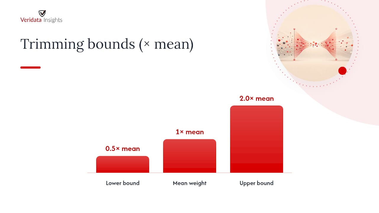
Common trimming bounds run somewhere around 0.5 to 2.0 times the mean weight, though the right bound depends heavily on your sample size and how skewed your base weights already are. Larger or more heterogeneous samples sometimes need tighter bounds; smaller studies can often tolerate looser ones.
On software, you have real options depending on your team’s existing stack:
- R’s survey package handles post-stratification, raking, and design-based variance estimation, and it’s free, which matters for smaller shops
- Stata’s
svysuite covers similar ground with a syntax many applied researchers already know - SAS and SUDAAN remain standard in government and large institutional research settings, particularly where replicate-weight methods are required
Guidance from Columbia’s Mailman School on constructing complex weights recommends exactly this kind of layered, software-documented approach rather than ad hoc spreadsheet adjustments.
Pro Tip: Version your weighting code the same way you’d version any other analysis script, and archive the intermediate weight files at each stage (base, nonresponse-adjusted, calibrated). When a client asks six months later why a number changed, you want to be able to answer in minutes, not days.
If your diagnostics keep flagging problems no matter how you adjust the weighting scheme, that’s usually a signal the issue is upstream in the sample design itself, and it’s worth consulting a methodologist before pushing weights further.
A Worked Outline: Building Weights Step by Step
Here’s how the sequence plays out on an actual project, stripped down to the decision points that matter:
- Calculate base weights from the sampling design, taking the inverse of each unit’s known selection probability. Stratified designs get stratum-specific base weights; simple random samples get a single uniform base weight.
- Adjust for nonresponse within response-rate strata, inflating weights for respondents in low-response groups so they represent the nonresponders in that same group.
- Calibrate or rake to population margins, whether that’s a single-dimension post-stratification against one benchmark or a multi-variable raking scheme against several margins simultaneously.
- Inspect the resulting weight distribution, trim or bound outliers as needed, recalculate effective sample size, and rerun your key topline estimates under both the weighted and unweighted schemes to confirm the adjustment is doing what you expect.
Every step should leave a paper trail. If a reviewer or client asks why a number moved between an interim and final report, the answer should be sitting in your documentation, not in your memory.
Why Methodology Comes First at Veridata Insights
Weighting can only fix so much. Data you trust starts with design decisions made before a single response comes in, which is why Veridata Insights treats weighting as one link in a longer chain rather than a fix applied at the end. Good sampling and questionnaire design reduces how much correction your weights need to carry in the first place.
A few things worth knowing before you bring in outside help on a weighting problem:
- Complex designs with multiple strata, hard-to-reach populations, or nonprobability panels usually justify a specialist’s eye, not a spreadsheet formula
- The right starting question is almost always about sample size and structure, covered in our breakdown of how many respondents you actually need
- A full-service weighting engagement should include diagnostics, not just a weighting scheme handed over cold
That’s the standard a methodology-first shop holds itself to, whether it’s a Fortune 500 tracking study or a niche B2B panel of forty respondents.
Get Defensible Weights Without Building an In-House Statistics Team
Building a defensible weighting scheme in-house means someone on staff who can run design effects, defend trimming bounds, and explain a raking convergence failure to a skeptical stakeholder. Not every research team has that person sitting free, and hiring one just for a single study rarely makes financial sense.
A full-service weighting engagement should include the full sequence: design weights, nonresponse adjustment, calibration, plus diagnostics that assess the need for weighting, delivered as part of a single engagement with flexible support options. This is especially important for complex designs such as multi-country studies, hard-to-reach populations, and nonprobability panels where propensity weighting and sensitivity checks are critical to producing defensible estimates.
If your next study involves a weighting scheme you don’t want to defend alone, reach out to our team to talk through methodology, programming, and diagnostics before your fieldwork even closes.
Sources
- Survey weights explained (Understanding Society blog)
- How different weighting methods work (Pew Research Center)
- Construction of complex survey weights (Columbia University Mailman School)
- Census