

When your sample is small, skip the reflexive p-value hunt. Prioritize effect sizes with confidence or credible intervals, lean on resampling or Bayesian methods when the design allows it, and use t-based tests carefully rather than defaulting to rank tests, which lose power fast at low n. Treat single hypothesis tests as premature until you’ve run at least one corroborative analysis. The BMJ, NCBI’s small clinical trials review, and Veridata Insights’ own project work all point the same direction: estimate, don’t just test.
TL;DR:
- Effect sizes with confidence or credible intervals are more informative than p-values in small samples, especially when using Bayesian or resampling methods.
- T-distribution-based tests, such as paired t-tests, typically outperform rank-based nonparametric tests at very low n, provided the data are close to normal.
- Proper study design choices like sequential analysis, repeated measures, hierarchical models, and finite population correction can significantly increase reliability with small samples.
- Using bootstrap, permutation, or Bayesian approaches helps validate results, but small n still limits the ability to detect subtle effects or generalize findings.
- Reporting effect sizes and intervals, along with corroborative analyses, ensures more honest, reproducible conclusions than relying solely on p-values.
Table of Contents
- What statistical methods actually work at very small n?
- How can you design a small study to get more reliable answers?
- Can bootstrap, permutation, or Bayesian methods rescue a tiny dataset?
- When should you trust parametric tests over nonparametric ones?
- How do you report results honestly when your sample is small?
- What does a defensible small-sample workflow actually look like?
- What mistakes quietly undermine small-sample results?
- Where can you go deeper on small-sample methods?
- How Veridata Insights supports small-sample projects
- Sources
What statistical methods actually work at very small n?
The instinct to switch to a “distribution-free” rank test the moment your sample looks thin is usually backwards. Nonparametric methods sound safer because they make fewer assumptions, but that safety comes at a steep cost in power. Mann-Whitney U cannot produce a p-value below 0.05 for groups smaller than four; Wilcoxon signed-rank hits the same wall below six, according to the Penn State case study on t-distribution methods. A test that mathematically cannot reach significance isn’t conservative. It’s just uninformative.
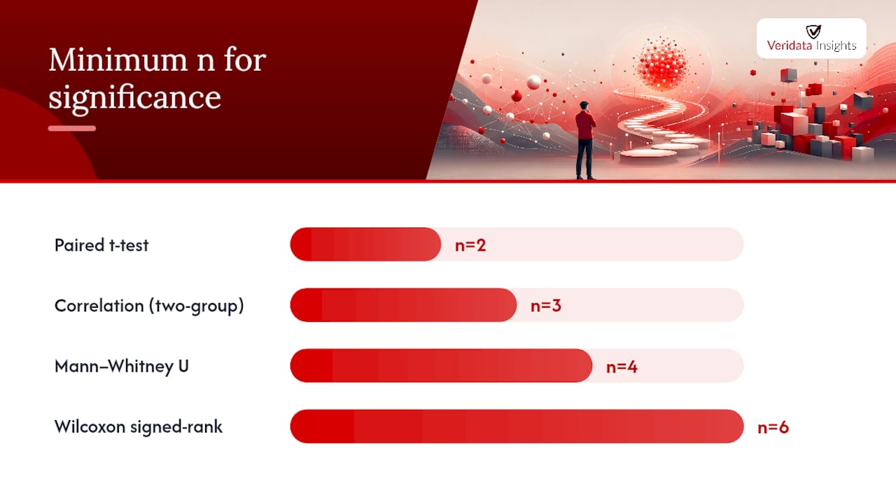
T-distribution-based methods, by contrast, can detect real differences with startlingly few observations. Paired t-tests have shown effective detection with n as small as 2, and correlation can be assessed in independent two-group comparisons with n=3, per the same Penn State analysis. The BMJ’s primer on continuous data from small samples backs this up with side-by-side comparisons: in several worked examples, a t-test flagged a difference that a rank-based equivalent simply could not detect, given the same data.
This doesn’t mean t-tests are always the right call. It means the common advice to “use nonparametric tests when n is small” gets the logic backwards. Rank tests need larger samples to achieve the same power a t-test gets from modeling the underlying distribution directly. If your data are reasonably close to normal, or you have prior knowledge suggesting they should be, a t-test is often the more defensible choice at low n, not the riskier one.
Where exact and count-based tests fit instead:
- Fisher’s exact test handles small 2×2 contingency tables (say, treatment success/failure across two groups of 5 to 10) without relying on large-sample chi-square approximations.
- Binomial tests work well for simple proportion questions: did 4 out of 6 trials succeed against a chance baseline?
- Poisson-based methods suit rare-event counts, like adverse events across a handful of clinical sites, where the outcome is a count rather than a continuous measure.
- Exact permutation-based rank tests (rather than their asymptotic p-value approximations) can partially rescue nonparametric methods at small n, though they still need enough distinct data arrangements to produce a meaningful p-value.
A few quick decision rules help here. For paired designs (pre- / post-measurements on the same 2 to 6 subjects), a paired t-test is usually your strongest option if the differences look roughly symmetric; if they’re heavily skewed, a sign test is a fallback, though it sacrifices power. For small independent groups (n≈3 to 8 per arm), check whether the outcome is continuous or categorical first. Continuous and roughly normal: t-test. Binary: Fisher’s exact. Count-based: Poisson or negative binomial, depending on overdispersion.
Consider a pharma-adjacent example: a pilot study comparing symptom scores before and after a short intervention in six patients. A paired t-test can detect a consistent shift even at n=6, provided the differences aren’t wildly skewed by one outlier. Compare that to a Wilcoxon signed-rank test on the same data. It literally cannot return p<0.05 with fewer than six pairs, so if your n is 5, you’ve already lost the ability to find significance regardless of the true effect. That’s not a hypothetical concern. It’s a mechanical limit built into the test’s ranking structure.
The takeaway for method selection isn’t “parametric good, nonparametric bad.” It’s that method choice should follow from what you know about the data-generating process, not from a rule of thumb that treats small n as automatically disqualifying for parametric approaches.
How can you design a small study to get more reliable answers?
Method choice matters, but design choices made before you collect a single data point often matter more. A well-designed study with 20 subjects can out-inform a sloppy one with 80.
- Consider a sequential design. Rather than fixing n in advance, sequential designs let you evaluate accumulating data at pre-specified checkpoints and stop early when results are clear. The NCBI Bookshelf review of small clinical trial analysis notes that sequential approaches tend to reduce the average sample size needed to reach a conclusion, compared with fixed-n designs, though they require a documented stopping rule set in advance. Without one, you’re just p-hacking with extra steps.
- Use repeated measures or crossover designs wherever the outcome allows it. Measuring the same subject under multiple conditions removes between-subject variability from your error term entirely. A crossover design with 10 participants can rival the power of a parallel-group study with two to three times as many, simply because each person acts as their own control.
- Borrow strength through hierarchical or pooled models. If you’re running a multi-site pilot with 8 subjects per site across 4 sites, a hierarchical model that partially pools site-level estimates toward a common mean gives you more stable estimates than analyzing each site in isolation. The NCBI review specifically recommends hierarchical models for small clinical trials as a way to increase the information extracted from limited data.
- Apply finite population correction when your target population is genuinely small. This is the design fix analysts most often forget. If you’re studying a population of 200 (a rare disease cohort, a specific job role within one company), the sample size math changes. A Pearson sample-size calculator example shows a study that would normally need 150 subjects in an unbounded population dropping to about 86 subjects once you apply finite population correction for a population capped at 200. If you’re recruiting from a bounded pool and still using infinite-population formulas, you’re likely overestimating how much data you need.
- Protect measurement precision before you protect sample size. Pretesting your instrument on even 3 to 5 pilot subjects to catch ambiguous wording or scaling problems reduces measurement error, which does more for your effective power than adding a few more bodies to a noisy instrument.
- Plan for attrition explicitly. In a small study, losing even 2 participants can gut your usable n by 20% or more. Build in a buffer during recruitment, and decide upfront how you’ll handle dropouts analytically rather than deciding after you see which direction the missing data breaks.
Good sample size planning starts well before data collection, and thoughtful recruitment strategy determines whether your final n is usable at all or full of half-completed responses you’ll have to discard.
Can bootstrap, permutation, or Bayesian methods rescue a tiny dataset?
Resampling and Bayesian methods often outperform classical large-sample techniques precisely because they don’t assume you have a lot of data to begin with. That’s not a workaround. It’s the whole point of the approach.

Bootstrap confidence intervals work by resampling your observed data (with replacement) thousands of times to build an empirical distribution of your statistic, rather than relying on a theoretical formula that assumes a specific shape. This stabilizes estimates nicely when your sample, however small, is reasonably representative of the population you care about. The catch: if your original 8 to 10 observations happen to miss an entire subgroup or fail to capture the tail behavior of the underlying distribution, the bootstrap will faithfully reproduce that blind spot in every resample. Bootstrapping amplifies what’s in your data. It cannot invent what isn’t there.
Permutation tests suit designs where, under the null hypothesis, group labels are exchangeable. If you’re comparing two treatment arms of 6 patients each, a permutation test recalculates your test statistic across every possible relabeling of which patient belongs to which group, building an exact null distribution from your actual data rather than an asymptotic approximation. This makes permutation tests one of the more defensible options for small, tightly controlled experimental comparisons, since they don’t lean on large-sample theory at all.
Bayesian hierarchical models and empirical-Bayes methods take a different route: they let you borrow information across related groups or from prior studies, shrinking noisy small-sample estimates toward a more stable pooled estimate. The PMC review on small sample sizes in high-dimensional data analysis points to regularization and information-borrowing approaches as necessary tools once your sample size gets small relative to the number of parameters you’re estimating. This is especially relevant in genomics, psychometrics, and any field where you’re measuring many variables on few subjects.
If you go Bayesian, prior sensitivity isn’t optional disclosure. It’s part of the result.
- Report at least two plausible priors (a weakly informative one and a more skeptical one) and show whether your conclusion holds across both.
- If a result only survives under one specific prior choice, say so explicitly rather than reporting only the most favorable version.
- Pair any Bayesian estimate with its credible interval, not just a point estimate.
Pro Tip: Run your primary analysis through at least two different plausible methods, say, a t-test and a bootstrap CI, on the same small dataset. If they agree, you’ve got corroborative evidence. If they diverge sharply, that disagreement itself is a finding worth reporting, not a problem to bury.
Corroborative analysis is one of the cheapest credibility boosts available to a small-sample researcher. Running two or three defensible methods and reporting where they converge (or don’t) gives readers a far better sense of how solid your conclusion actually is than a single p-value ever could.
When should you trust parametric tests over nonparametric ones?
Small samples make it hard to check assumptions the normal way. You can’t eyeball a histogram of 7 data points and confidently declare normality one way or the other. That doesn’t mean you’re stuck guessing.
A few diagnostics still earn their keep even at low n:
- Difference plots for paired data. Plotting the raw pre- / post-differences (rather than the two original series separately) often reveals skew or outliers that a formal normality test, itself underpowered at small n, would miss entirely.
- Skew and symmetry checks. A simple visual check of whether your differences cluster roughly symmetrically around zero tells you more than a Shapiro-Wilk test run on 6 observations, where the test itself has almost no power to detect non-normality.
- Influence and leverage diagnostics. In a dataset of 10 points, a single outlier can single-handedly flip your conclusion. Calculating Cook’s distance or simply rerunning the analysis with each point excluded one at a time (a leave-one-out check) shows you exactly how fragile your result is.
External knowledge often matters more than in-sample diagnostics when n is this low. If you’re measuring a variable that’s well established in prior literature to be approximately normal (height, blood pressure, standardized test scores), you have legitimate grounds to use a parametric method even though your own 8 data points can’t confirm normality on their own. This is a case where domain knowledge should override a mechanical assumption check that has no statistical power to begin with.
If assumptions genuinely fail, or you have real reason to doubt them, you have options short of abandoning inference altogether:
- Transform the data. A log transform on right-skewed count or duration data often restores enough symmetry to justify a t-test.
- Fall back to a sign test for paired data when differences are badly skewed. You lose power, but you gain robustness against distributional assumptions.
- Use robust estimators like the trimmed mean or Huber M-estimator, which reduce the influence of outliers without requiring you to discard data points outright.
None of these fixes require you to reflexively grab a rank-based test the moment your n drops below 20. Match the fix to the specific way your assumptions failed, not to a blanket small-sample rule.
How do you report results honestly when your sample is small?
A p-value from an eight-person study tells you almost nothing about whether an effect is real or how large it is. Effect size, and the uncertainty around it, is the actual finding. Report that first.
Power calculations still have a role, but only on the front end. Calculating power during study planning helps you decide whether a study is even worth running, or how many corroborative data sources you’ll need to make the result credible. Calculating “post-hoc power” after you already have your p-value is close to meaningless. It’s mathematically just a rescaled version of the p-value you already computed, dressed up to look like new information.
What responsible reporting looks like in practice:
- Lead with the effect size (mean difference, odds ratio, correlation coefficient) and its confidence or credible interval, not the p-value.
- Show the interval visually where possible. A forest plot or simple interval plot communicates uncertainty far better than a table of point estimates.
- State explicitly whether the study was designed to test a hypothesis or to generate one. A small pilot generating a hypothesis for a larger confirmatory study is legitimate science. A small pilot presented as confirmatory evidence is not.
- Flag findings as preliminary when they haven’t been corroborated by at least one alternative method or independent dataset.
A confidence interval that runs from a small negative effect to a large positive one is not a failed result. It’s an honest one. Reporting it that way, instead of chasing a point estimate past a significance threshold, is what separates defensible small-sample research from noise dressed up as a discovery.
The NCBI Bookshelf’s guidance on small clinical trials makes a related point: because small trials generate limited information per study, running corroborative analyses (a secondary endpoint check, a sensitivity analysis, a replication in a related dataset) adds real evidentiary weight in a way that squeezing a single dataset harder never can. If two independently reasonable analytic approaches on the same small dataset land on the same conclusion, you have something worth reporting. If they don’t, you have an important caveat, not a result to hide.
What does a defensible small-sample workflow actually look like?
At Veridata Insights, we’ve supported research teams across pharmaceutical, B2B, and hard-to-reach healthcare studies where the final analyzable n rarely cracks three digits. The pattern that produces defensible results is consistent enough to write down as a checklist.
- Define the estimand before touching the data. What effect, specifically, are you trying to estimate? Vague research questions produce vague, unfalsifiable analyses.
- Pre-register your primary analysis method. Decide on your test or model before you see the results, especially at small n where the temptation to try five methods and report the best-looking one is strongest.
- Check design-stage fixes. Can you use a repeated-measures structure? Does finite population correction apply? Is a sequential stopping rule appropriate?
- Run diagnostics on the raw data first. Difference plots, skew checks, and outlier flags, before you pick a test.
- Run your primary analysis, plus at least one corroborative method. A t-test alongside a bootstrap CI, for instance.
- Report effect sizes and intervals, not bare p-values.
- Run a leave-one-out sensitivity check to see how fragile your conclusion is to any single observation.
- Document every deviation from your pre-registered plan, and label any additional analyses as exploratory.
- Produce a reproducible artifact, a notebook or script, not just a results table, so the analysis can be audited or extended.
- Write an interpretation memo that states plainly what the data do and don’t support.
This is where a full-service research partner earns its keep, particularly at the front and back ends of that list. Veridata Insights works with research teams on the pieces that determine whether a small-n study is usable at all: questionnaire review to catch measurement problems before data collection starts, recruitment for hard-to-reach B2B and healthcare audiences where n=15 might represent a genuinely difficult-to-source population, survey programming, and reporting that visualizes uncertainty instead of hiding it behind a single asterisk.
If you’re evaluating a vendor for a small-sample project, ask for these deliverables specifically:
- A codebook documenting every variable, its coding, and any transformations applied.
- A reproducible notebook or script, not just a static output file.
- A sensitivity appendix showing how results shift under alternative reasonable methods.
- A plain-language interpretation memo that states the estimand, the finding, and its limitations without overclaiming.
Vendors who resist providing any of these are usually hiding either sloppy methodology or a result that doesn’t hold up to a second look.
What mistakes quietly undermine small-sample results?
A handful of errors show up again and again in small-n analyses, and most of them are catchable with a five-minute check.

Overfitting and unstable coefficients. If you’re fitting a regression with 6 predictors on 25 observations, your model is memorizing noise, not detecting signal. A GitHub-hosted methodology repository analyzing supervised learning workflows for n≈30 to 200 found that simple penalized models (ridge regression) consistently outperformed more flexible ensemble methods at small n, largely because ensembles overfit fast when data are scarce. The practical fix: enforce a feature budget, roughly one predictor for every 10 to 15 observations, and prefer ridge or lasso regression over anything more flexible until your sample grows. Watch for wild coefficient swings across cross-validation folds; that instability is your overfitting alarm.
Multiple testing and data snooping. Running 15 exploratory comparisons on a 20-person dataset and reporting only the 2 that hit p<0.05 is the fastest way to produce a false discovery. Pre-specify your primary analyses, and report anything else explicitly as exploratory, not confirmatory.
Missing data handling. Multiple imputation, the standard fix for missing data in large samples, can behave erratically with small n because it needs enough observed data to model the missingness pattern credibly. Full-information maximum likelihood (FIML) or a simple sensitivity analysis comparing complete-case results against imputed results is often more transparent at small n than a black-box imputation procedure.
Skipping robustness checks entirely. A leave-one-out analysis, rerunning your model 8 times, once with each observation dropped, takes minutes and tells you immediately whether your conclusion depends on a single data point. If dropping any one observation flips your result, you don’t have a finding yet. You have a fragile pattern that needs more data before it’s reportable.
Pro Tip: Before you write up any small-sample result, rerun it with your largest outlier removed. If your conclusion survives, say so in the write-up. If it doesn’t, that’s not a footnote, it’s the headline finding about your data’s reliability.
Where can you go deeper on small-sample methods?
A short list of resources covers most of what a working analyst needs beyond this article. The BMJ’s primer on continuous data from small samples is the fastest read for understanding t-test versus rank-test tradeoffs. The NCBI Bookshelf chapter on small clinical trials goes deeper on hierarchical models and sequential design. The PMC review of high-dimensional small-sample problems is the right reference once your variable count starts approaching your sample size. The Penn State case study offers worked numerical examples you can replicate by hand. For synthesizing results across multiple small studies, PaperSynapse’s guide to evidence tables walks through structuring evidence comparisons so corroborative findings are easy to weigh side by side.
How Veridata Insights supports small-sample projects
Full-service market research doesn’t stop being useful just because your n is small. It matters more. Veridata Insights runs methodology consultation, questionnaire review, and recruitment for B2B, healthcare, and other hard-to-reach audiences where a defensible sample of 30 takes more craft than a convenience sample of 3,000. Every engagement includes programming, data processing, and reporting built for reproducibility: codebooks, sensitivity checks, and interpretation memos, not just a results deck. There are no project minimums, and the team works seven days a week, so a tight research timeline doesn’t force you to cut corners on a study where every observation counts. If your next project depends on getting real answers from a limited sample, get in touch with Veridata Insights to scope the recruitment, analysis, or reporting support you need.
Sources
- Analysis of continuous data from small samples | The BMJ
- Small sample sizes: A big data problem in high-dimensional data analysis (PMC review)
- Statistical approaches to analysis of small clinical trials (NCBI Bookshelf)
- Small-sample t-distribution guidance (PSU stat case study)